Multi-angle MaxCut QAOA#
This tutorial illustrates how to use paulie to classify the dynamical Lie algebra (DLA)
of the multi-angle MaxCut Quantum Approximate Optimization Algorithm (QAOA) ansatz, reproducing the
six-family result of Kazi et al. [2025] and the classification shown in Figure 8 of
Shaya et al. [2025].
The ansatz and its Lie algebra#
For a connected graph \(G = (V, E)\) on \(n = |V|\) qubits, the multi-angle (also called free) MaxCut QAOA ansatz assigns an independent angle to every generator in
Each \(X_v\) is the Pauli string carrying \(X\) on qubit \(v\) (e.g. XII) and each
\(Z_u Z_v\) carries \(Z\) on the two endpoints of an edge (e.g. ZZI). The object we
classify is the DLA, the real span of these generators together with all of their nested
commutators,
The six connected graph families and their Lie algebras#
The six families are distinguished by standard properties of the graph. A graph is bipartite if its vertices split into two sets, its two parts, so that every edge joins one part to the other (equivalently, it contains no odd-length cycle). Among the graphs used below, a path \(P_n\) joins \(n\) vertices in a line, a cycle \(C_n\) joins them in a closed loop, the complete bipartite graph \(K_{a,b}\) joins every vertex of one part of size \(a\) to every vertex of the other of size \(b\), and the complete graph \(K_n\) joins every pair of its \(n\) vertices.
Kazi et al. [2025] prove that, for any connected graph, the multi-angle DLA falls into exactly one of six families, determined by these properties. A graph is called archetypal when it is connected but neither bipartite nor a cycle graph; the even–even, odd–odd and even–odd labels refer to the parities of the sizes of the two parts of a connected bipartite graph.
The animation below shows the maximum cut for a representative of different graph families: a red cut line separates the two vertex groups and crosses the cut edges. A bipartite graph has a cut that crosses every edge, whereas a non-bipartite graph always leaves some edges uncut.
Graph family |
Bipartite? |
\(\dim\,\mathfrak{g}_\mathrm{free}\) |
Lie algebra \(\mathfrak{g}_\mathrm{free}\) |
|---|---|---|---|
Path |
yes |
\(2n^2 - n\) |
\(\mathfrak{so}(2n)\) |
Cycle |
if \(n\) even |
\(4n^2 - 2n\) |
\(\mathfrak{so}(2n) \oplus \mathfrak{so}(2n)\) |
Even–even |
yes |
\(2^{2n-2} - 2^{n-1}\) |
\(\mathfrak{so}(2^{n-1}) \oplus \mathfrak{so}(2^{n-1})\) |
Odd–odd |
yes |
\(2^{2n-2} + 2^{n-1}\) |
\(\mathfrak{sp}(2^{n-1}) \oplus \mathfrak{sp}(2^{n-1})\) |
Even–odd |
yes |
\(2^{2n-2} - 1\) |
\(\mathfrak{su}(2^{n-1})\) |
Archetypal |
no |
\(2^{2n-1} - 2\) |
\(\mathfrak{su}(2^{n-1}) \oplus \mathfrak{su}(2^{n-1})\) |
Note
The six-family result is specific to the multi-angle (free) ansatz. Thus, the classification should not be extended to QAOA in general.
Diagnosing barren plateaus#
The dimension of the DLA controls how the cost-function gradients scale, and therefore whether a variational circuit can be trained. When this dimension grows exponentially with the number of qubits \(n\), the gradient variance vanishes exponentially, which is the barren-plateau condition (Kazi et al. [2025], Corollary 2; Shaya et al. [2025]). For the multi-angle MaxCut ansatz, every family except the path and cycle has an exponentially large DLA (see the table above), so those circuits are extremely prone to barren plateaus even at a single layer, whereas the polynomially small path and cycle families may instead be classically simulable. Classifying the DLA therefore diagnoses in advance whether the variational circuit is trainable.
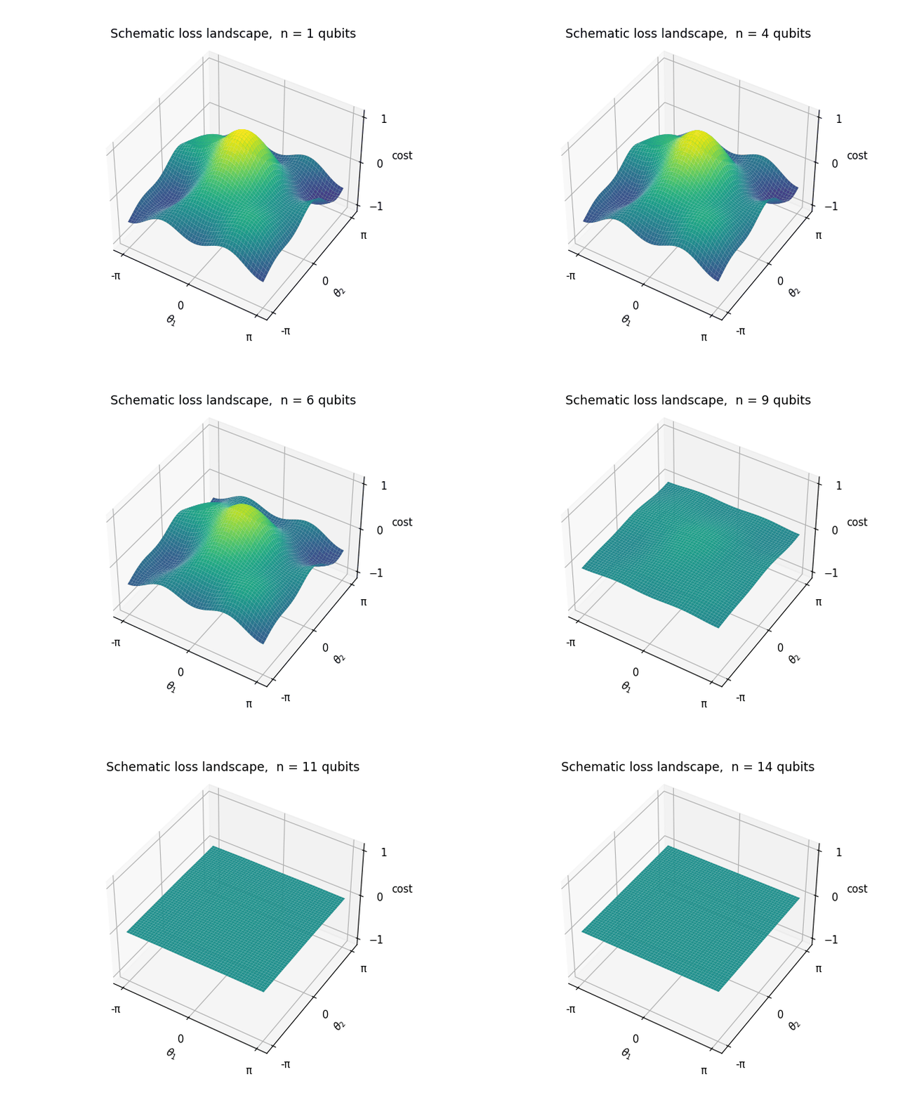
As an illustration, the animation below shows schematically how the loss landscape flattens as the number of qubits increases for the exponentially large families (even–even, odd–odd, even–odd, and archetypal): the gradients shrink until the landscape becomes an almost flat barren plateau.
Reproducing the classification#
The six-family result can be reproduced with paulie alone, by giving it the generators of a
small representative of each family as Pauli strings:
from paulie import get_pauli_string as p

families = {
    "path P3":        ["XII", "IXI", "IIX", "ZZI", "IZZ"],
    "cycle C4":       ["XIII", "IXII", "IIXI", "IIIX", "ZZII", "IZZI", "IIZZ", "ZIIZ"],
    "even-odd K1,4":  ["XIIII", "IXIII", "IIXII", "IIIXI", "IIIIX",
                       "ZZIII", "ZIZII", "ZIIZI", "ZIIIZ"],
    "odd-odd K1,3":   ["XIII", "IXII", "IIXI", "IIIX", "ZZII", "ZIZI", "ZIIZ"],
    "archetypal K4":  ["XIII", "IXII", "IIXI", "IIIX",
                       "ZZII", "ZIZI", "ZIIZ", "IZZI", "IZIZ", "IIZZ"],
    "even-even K2,4": ["XIIIII", "IXIIII", "IIXIII", "IIIXII", "IIIIXI", "IIIIIX",
                       "ZIZIII", "ZIIZII", "ZIIIZI", "ZIIIIZ", "IZZIII", "IZIZII", "IZIIZI", "IZIIIZ"],
}
for name, gens in families.items():
    g = p(gens)
    print(f"{name}: {g.get_algebra()}, dim {g.get_dla_dim()}")
outputs
path P3: so(6), dim 15
cycle C4: 2*so(8), dim 56
even-odd K1,4: su(16), dim 255
odd-odd K1,3: 2*sp(4), dim 72
archetypal K4: 2*su(8), dim 126
even-even K2,4: 2*so(32), dim 992
Each line reproduces the corresponding row of the table above. The path gives a single
\(\mathfrak{so}\) algebra and the cycle a sum of two, both of polynomial dimension; the even-odd
graph gives \(\mathfrak{su}\), the odd-odd graph \(\mathfrak{sp}\), and the even-even and
archetypal graphs sums of \(\mathfrak{so}\) and \(\mathfrak{su}\), all of exponential
dimension. The smallest case is checkable by hand: the path \(P_3\) gives \(\mathfrak{so}(6)\)
of dimension \(2n^2 - n = 15\) at \(n = 3\). (paulie writes a direct sum of two
identical factors with a numeric prefix, so 2*so(8) is \(\mathfrak{so}(8) \oplus
\mathfrak{so}(8)\).) For each family, paulie returns the algebra and dimension predicted by
Kazi et al. [2025]; Figure 8 of Shaya et al. [2025] shows this agreement across \(n = 4\) to
\(24\).
See also
For the algorithm behind get_algebra, see Classification of Pauli DLAs.