Classification of Pauli DLAs#
This tutorial will illustrate how to use paulie to classify the dynamical Lie algebra of a circuit given
the generators consisting of Pauli strings.
A Pauli string is a tensor product of Pauli matrices
and is represented as a string indicating the Pauli matrices successively. Given a set of Pauli strings, the closure under the commutator defines a Lie algebra.
In Aguilar et al. [2024], an efficient algorithm for classifying which Lie algebra is generated is given. PauLie implements
a modified version of this algorithm.
The function get_algebra returns exactly which algebra is generated when
given the generator set which can be extended with identities to arbitrary qubit numbers
specified.
We can reproduce Example I.5 in Wiersema et al. [2024]:
from paulie import get_pauli_string as p

generators = p(["XY"])
algebra = generators.get_algebra()
print(f"algebra = {algebra}")
outputs
algebra = u(1)
whereas changing to a three qubit system, results in another algebra:
size = 3
generators = p(["XY"], n=size)
algebra = generators.get_algebra()
print(f"algebra = {algebra}")
outputs
algebra = so(3)
The algorithm is based on the concept of an anticommutation graph. Given a set of n-qubit Pauli strings \(\mathcal{G} = \{P_1,\dots ,P_{n_G}\}\), the anticommutation graph has as a vertex set \(\mathcal{G}\) and edges between all vertices that do not commute. The fundamental operation we use is a contraction between two Pauli strings \(P_i\) and \(P_j\) which maps \(P_i \mapsto \pm \frac{1}{2} i [P_i,P_j] = P_i^\star\). Crucially, it can be shown that this operation leaves the Lie algebra invariant. Now if \(P_i^\star\) is already in \(\mathcal{G}\), the size of the generator set has been reduced. Otherwise, the operation results the complementation of the edge set between \(P_i^\star\) and vertices in the neighbourhood of \(P_j\). Simply put, we can use such contractions to manipulates the edges of the anticommutation graph so as to bring it to a canonical form.
For any generator set consisting of Pauli strings, the anticommutation graph can be transformed to four canonical types (Theorem 1 in Aguilar et al. [2024]). Each canonical type corresponds to a particular algebra. There is an exception if \(\mathcal{P}\) only has one Pauli string. A single Pauli string generates the algebra \(\mathfrak{u}(1)\).
Canonical type |
Structure |
Lie algebra |
|---|---|---|
A |
\(\left|N\right| = n_1\), \(\left|T\right| = 0\), \(\left|L^{\mathcal{B}}\right| = n\) |
\(\bigoplus_{i=1}^{2^{n_1}}\mathfrak{so}(n + 3)\) |
B1 |
\(\left|N\right|=n_1\), \(\left|T\right| = n_2\), \(\left|L^{\mathcal{B}}\right|=0\) |
\(\bigoplus_{i=1}^{2^{n_1}}\mathfrak{sp}(2^{n_2})\) |
B2 |
\(\left|N\right|=n_1\), \(\left|T\right| = n_2\), \(\left|L^{\mathcal{B}}\right|=4\) |
\(\bigoplus_{i=1}^{2^{n_1}}\mathfrak{so}(2^{n_2 + 3})\) |
B3 |
\(\left|N\right|=n_1\), \(\left|T\right| = n_2\), \(\left|L^{\mathcal{B}}\right|=3\) |
\(\bigoplus_{i=1}^{2^{n_1}}\mathfrak{su}(2^{n_2 + 2})\) |
Visualizing the transformation#
The step-by-step transformation of the anticommutation graph into its canonical form can be
animated with animation_anti_commutation_graph. It drives the classification algorithm
through a recording wrapper that observes every step (without changing the result) and renders the
captured frames into an animation:
from paulie import get_pauli_string as p, animation_anti_commutation_graph

generators = p(["XY", "XZ"], n=4)
animation_anti_commutation_graph(
    generators,
    storage={"filename": "classification.gif", "writer": "pillow"},
)
Each frame highlights the role a vertex currently plays, following this colour legend:
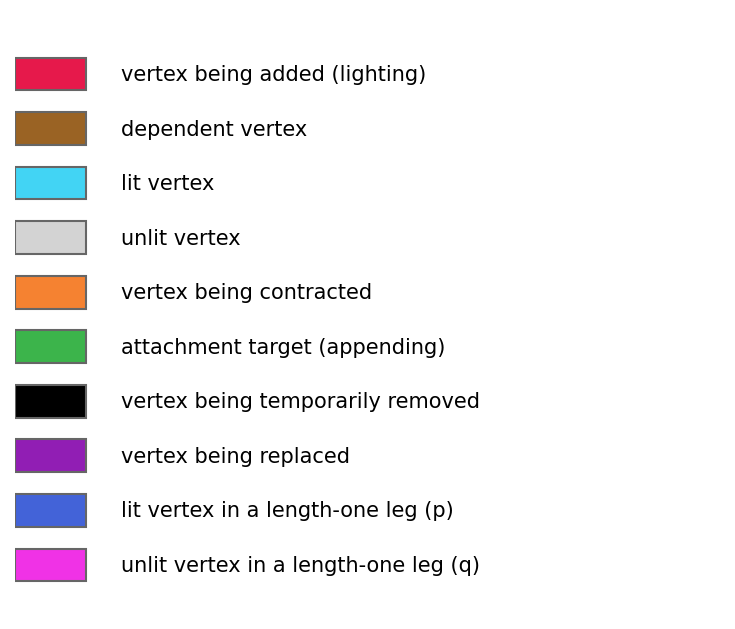
The two worked examples below are illustrated with interactive players. Use the controls to play, pause, or step through the construction frame by frame.
Classification of A-type canonical graph#
Let’s try to classify a generator set that corresponds to an A-type canonical graph. This algebra is generated by \(\mathcal{P}=\{IYZI,IIXX,IIYZ,IXXI,XXII,YZII\}\).
generators = p(["IYZI", "IIXX", "IIYZ", "IXXI", "XXII", "YZII"])
algebra = generators.get_algebra()
print(f"algebra = {algebra}")
outputs
algebra = 4*so(5)
The player below follows the construction of one of the four canonical components. Starting from
the input anticommutation graph, each generator is added in turn (red), attached to the centre or to
a leg (green), and length-one legs in different lit states are merged using the p (blue) and
q (pink) vertices, until the A-type star graph is obtained:
According to the table, the resultant graph corresponds to \(\mathfrak{so}(5)\oplus \mathfrak{so}(5)\oplus \mathfrak{so}(5)\oplus \mathfrak{so}(5)\). But it is worth noting that it also corresponds to \(\mathfrak{sp}(2)\oplus \mathfrak{sp}(2)\oplus \mathfrak{sp}(2)\oplus \mathfrak{sp}(2)\). This shows that there is an exceptional isomorphism between \(\mathfrak{so}(5)\) and \(\mathfrak{sp}(2)\).
Classification of B-type canonical graph#
Let’s try to classify a generator set that corresponds to a B-type canonical graph, that is a anticommutation graph that is a star graph. We demonstrate it by the algebra \(\mathfrak{a}_9\) [1], generated by \(XY\) and \(XZ\).
n_qubits = 4
generators = p(["XY", "XZ"], n=n_qubits)
algebra = generators.get_algebra()
print(f"algebra = {algebra}")
outputs
algebra = sp(4)
Here the contractions reduce the graph to a single long leg attached to the centre, the canonical form of type B1 corresponding to \(\mathfrak{sp}(4)\):
Extracting the Underlying Matrix Basis#
This section shows how to extract its explicit matrix representation using the get_algebra_basis() method.
Note that we are reusing previous examples.
Example 1
from paulie import get_pauli_string as p

# Generates a 3D array of shape (3, 3, 3)
basis = p(["XY"], n=3).get_algebra_basis()
print(f"Basis contains {len(basis)} matrices of shape {basis[0].shape}")
outputs
Basis contains 3 matrices of shape (3, 3)
Example 2
from paulie import get_pauli_string as p

# This system compiles to a direct sum of four so(5) algebras
generators = p(["IYZI", "IIXX", "IIYZ", "IXXI", "XXII", "YZII"])
basis = generators.get_algebra_basis()

# Total elements: 4 summands * 10 generators each = 40
# Matrix size: 4 summands * 5x5 blocks = 20x20
print(f"Total basis elements: {len(basis)}")
print(f"Matrix dimensions: {basis[0].shape}")
outputs
Total basis elements: 40
Matrix dimensions: (20, 20)
The Lie algebra plays a pivotal role in quantum control theory to understand the reachability of states.
Also measures of operator spread complexity rely on this concept.
Furthermore, determining moments of circuits can be significantly simplified when the Lie algebra is known.
All these applications are functionalities of paulie.